

Abstract
This article illustrates how one might tackle AB-testing in a full Bayesian framework. In particular it compares the Evidence for a model which distinguishes between the coins with a model which lumps them together. This appears to be a good way to decide whether to explore the coins’ properties or exploit our existing knowledge.
AB-testing
The aim of AB-testing1 is to decide which of two alternatives is better. These days the classic example is which of two adverts a website should display, in days gone by we might ask which of two coins is more likely to land heads-up. Looking forward, and generalizing to the case of many choices, it is a key issue in Monte Carlo tree search2 where we have to decide which branch of the search tree to explore. We will usually talk about coins in the discussion below, but we’ll be tossing them in an environment which rewards us for getting heads.
There are two different problems to consider. In the first, we seek to make the best inference from a fixed set of data: as with all inferences this means we will apply Bayes’ theorem3.
In the second problem, we seek an algorithm which decides which coin to toss so as to maximize the number of heads at the end of the day. It seems likely that we will want to infer things here, but having made the inferences we will need to make decisions based on them too. Often there will be a tension between exploring the choices we have available to us, and exploiting the best choice.
In this article, we marry a careful Bayesian inference to very simple decision rules. The inference explicitly includes the case where our data prefer to not distinguish between the alternatives. These algorithms are conceptually straightforward and easy to think about, and perform reasonably well in synthetic experiments.
We limit our comparisons to just two coins, though it could be extended to more alternatives with a bit of thought.
Preliminary demonstrations
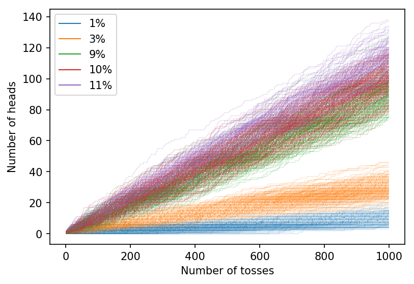
To get a feel for the problem look at the graph below which shows the number of heads seen from a thousand coin tosses.
We will use the phrase a ‘\(n\)% coin’ to mean a coin which has a probility \(n\)% of landing heads-up when tossed.
Five different coins are used: 1%, 3%, 9%, 10%, 11%. Coin tossing is a random business, and so the graph shows 1,000 samples of the thousand-toss experiment. For each sample, the coin is chosen at random, and so we expect about 200 traces for each coin.
 4
4
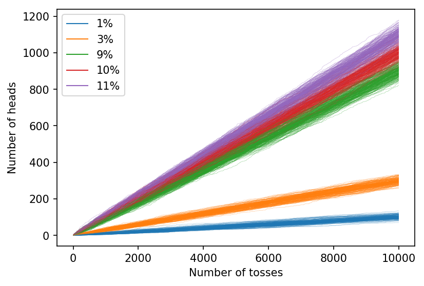
It is reasonably difficult to resolve the three different coins with probabilities \(0.09\), \(0.10\) and \(0.11\) on this graph, but things become clearer if we toss the coins for longer:
 5
5
Suppose you have 10%- and 11%-coins. It is clear from the graph that you’d need about 1,000 tosses to see much of a difference. Even if you tossed the coins 10,000 times, you couldn’t be sure that the coin which showed more heads was indeed more likely to show heads.
To be quantitative, after a large number \(n\) tosses where the chance of a head is \(p\) on each toss, the number of heads \(n_t\) is roughly Gaussian:
\[ n_t = n p \pm \sqrt{n p (1-p)}. \]Putting in some numbers, the table below shows the number of heads we expect to see expressed as mean and standard deviation:
| Coin | Number of tosses | |||
|---|---|---|---|---|
| 100 | 1,000 | 10,000 | 100,000 | |
| 9% | 9 ± 2.9 | 90 ± 9.0 | 900 ± 28.6 | 9,000 ± 90.5 |
| 10% | 10 ± 3.0 | 100 ± 9.5 | 1000 ± 30.0 | 10,000 ± 94.9 |
| 11% | 11 ± 3.1 | 110 ± 9.9 | 1100 ± 31.3 | 11,000 ± 98.9 |
Given two coins with probabilities \(p \pm \Delta p\), the one standard deviation points will match roughly when:
\[ \begin{eqnarray} \sqrt{n p (1-p)} &\approx& \frac{1}{2} n \, \Delta p, \\\ n &\approx& \frac{4 p (1-p)}{\Delta^2}. \end{eqnarray} \]Here \(p \approx 0.1, \Delta \approx 0.01 \) and so \(n \approx 3,600\), which is consistent with the demonstrations above. The details don’t matter, but it is important to realize that you’ll need a lot of tosses to resolve the difference between similar coins.
Basic Bernoulli Inference
In formal terms the standard model for tossing a coin is a Bernoulli process. Given the fixed probability of getting a head, \(p\), the likelihood of getting \(h\) heads in \(n\) tosses is
\[ \textrm{pr}(h|p) = \frac{n!}{h!(n-h)!} \, p^h\, (1-p)^{n-h}. \]We will generally assume a flat prior on \(p\), save for requiring it to be bounded by zero and one i.e.
\[ \textrm{pr}(p) = \begin{cases} 1 & \text{when } 0 \leq p \leq 1 \\\ 0 & \text{otherwise}. \end{cases} \]As an aside, note that some kinds of prior information can be encoded as a beta-function with hyper-parameters \(a\), and \(b\):
\[ \textrm{pr}(p|a,b) = \frac{(a + b + 1)!}{a!\, b!} p^a (1-p)^b. \]This function says that before I toss the coin it is as though I have already witnessed \(a\) heads and \(b\) tails: it is a reasonable way to encode \(p\) being roughly some value with a given precision. It is mathematically convenient because the prior has the same functional form as the likelihood, and so much of the algebra below is easy to extend.
There is no reason to limit \(a\) and \(b\) to being integers: if you do make this generalization then you need to replace the factorials with Gamma functions.
Returning to the flat prior on \(p\), and assuming everywhere that \(0 \leq p \leq 1\), we can calculate the joint distribution of \(p\) and \(h\):
\[ \textrm{pr}(p,h) = \frac{n!}{h! (n-h)!} p^{h} (1-p)^{n-h}. \]the Evidence,
\[ \begin{eqnarray} \textrm{pr}(h) &=& \int_0^1 \textrm{pr}(p,h) \, \textrm{d}p, \\\ &=& \frac{1}{n + 1}, \end{eqnarray} \]and the posterior,
\[ \textrm{pr}(p|h) = \frac{(n + 1)!}{h! (n-h)!} \; p^{h} (1-p)^{n-h}. \]It is helpful to write this in terms of the binomial coefficient,
\[ \textrm{pr}(p|h) = (n + 1) \, \binom{n}{h} \, p^{h} (1-p)^{n-h}. \]Two coins
Perhaps the simplest way to model AB-testing is to assume that A and B are completely independent. This means that all the variables above sprout a suffix indicating their allegiance, and the probabilities multiply.
For example the posterior distribution of \(p_A\) and \(p_B\) given the data:
\[ \begin{eqnarray} \textrm{pr}(p_A, p_B|h_A, h_B) &=& \textrm{pr}(p_A|h_A) \; \textrm{pr}(p_B|h_B) \\\ &=& (n_A + 1) \binom{n_A}{h_A} p_A^{h_A} (1-p_A)^{n_A-h_A} \; (n_B + 1) \binom{n_B}{h_B} p_B^{h_B} (1-p_B)^{n_B-h_B}, \\\ &=& (n_A + 1)(n_B + 1) \binom{n_A}{h_A} \binom{n_B}{h_B} \; p_A^{h_A} (1-p_A)^{n_A-h_A} \; p_B^{h_B} (1-p_B)^{n_B-h_B}. \end{eqnarray} \]To assess the probability that A is better than B just integrate the posterior over the region where \(p_A > p_B\):
\[ \textrm{pr}(p_A > p_B) = \int_0^1 \, \textrm{d}p_A \, \int_0^{p_A} \textrm{d}p_B \, \textrm{pr}(p_A, p_B|h_A, h_B). \]Sadly though this is messy:
\[ \textrm{pr}(p_A > p_B) = Q \int_0^1 \, \textrm{d}p_A \, \int_0^{p_A} \textrm{d}p_B \, p_A^{h_A} (1-p_A)^{n_A-h_A} \; p_B^{h_B} (1-p_B)^{n_B-h_B}, \]where \(Q\) denotes all the terms from above not involving \(p_i\). The integral is particularly hard in the cases that matter: if A and B are roughly as good as each other, the line \(p_A = p_B\) which marks one boundary of the area over which we are integrating will slice through a significant mass of probability.
That said, it is only a 2D-integral of a smooth function over a bounded region: solving it numerically is perfectly feasible for particular values of \(n_i\) and \(h_i\).
Happily, though, there is a better way to proceed.
Mr Inclusive
If we’re consciencious, we should compare the two-parameter model above with a simpler one-parameter model which assumes that both coins have the same chance of giving a head.
Bayesian model-comparison embodies an automatic Occam’s Razor6 which prefers simpler models unless the data provide a compelling reason to prefer a more complicated one. In the case of AB-testing we might hope that initially the simpler model will be preferred at first: essentially the good Reverend Bayes shrugs and says “I don’t have enough data to justify putting the coins in separate classes.”
Introducing \(\mathscr{H}_1\) for the 1-parameter hypothesis, the joint distribution is
\[ \begin{eqnarray} \textrm{pr}(h_1, h_2, p | \mathscr{H}_1) &=& \binom{n_A}{h_A} \, p^{h_A} (1-p)^{n_A-h_A} \; \binom{n_B}{h_B} \, p^{h_B} (1-p)^{n_B-h_B} \\\ &=& \binom{n_A}{h_A} \, \binom{n_B}{h_B} \; p^{h_A + h_B} \; (1-p)^{n_A + n_B - h_A - h_B}, \end{eqnarray} \]and thus the Evidence,
\[ \textrm{pr}(h_1, h_2 | \mathscr{H}_1) = \frac{1}{n_A + n_B + 1}\; \binom{n_A}{h_A}\, \binom{n_B}{h_B} \Big/ \binom{n_A + n_B}{h_A + h_B}. \]By contrast for the two-parameter model the Evidence is,
\[ \textrm{pr}(h_A, h_B | \mathscr{H}_2) = \frac{1}{(n_A + 1)(n_B+ 1)}. \]and thus, assuming we consider each possibility equally probable a priori,
\[ \begin{eqnarray} \frac{\textrm{pr}(\mathscr{H}_2|h_A, h_B)}{\textrm{pr}(\mathscr{H}_1|h_A, h_B)} &=& \frac{\textrm{pr}(h_A, h_B | \mathscr{H}_2)}{\textrm{pr}(h_A, h_B | \mathscr{H}_1)} \\\ &=& \frac{(n_A + 1)(n_B + 1)}{n_A + n_B + 1}\; \binom{n_A}{h_A}\, \binom{n_B}{h_B} \Big/ \binom{n_A + n_B}{h_A + h_B}. \end{eqnarray} \]If this ratio is bigger than one, the best inference is that the two coins have different probabilities with distribution:
\[ \textrm{pr}(p_A, p_B|h_A, h_B, \mathscr{H}_2) = \prod_{i \in \{A,B\}} (n_i + 1) \binom{n_i}{h_i} \; p_i^{h_i} (1-p_i)^{n_i-h_i}. \]otherwise we don’t distinguish the coins, and the single probability \(p\) with distribution,
\[ \textrm{pr}(p|h_A, h_B, \mathscr{H}_1) = (n_A + n_B + 1) \binom{n_A + n_B}{h_A + h_B} \; p^{h_A + h_B} \; (1-p)^{n_A-h_A + n_B - h_B}. \]Here endeth the inference.
An illustration
The expressions above are difficult to grasp intuitively, so instead we shall plot them! The plot below shows \(\textrm{pr}(\mathscr{H}_2|D)\) for different combinations of heads when two coins were each tossed 100 times.
 7
7
Areas in green are those where \(\mathscr{H}_2\) is more likely; those in purple favour \(\mathscr{H}_1\).
It is easy to see the symmetry between heads and tails, and between coins A & B. Also, note the relatively sharp transition between the two regimes.
Decision theory
The inferences above are the optimal conclusions to draw from a given set of data. If all we had were the results of a fixed experiment, we’d be done. However, suppose we can get more data. It is clear that we should do so both because we might learn more about the properties of the coins, but also we get rewarded for getting heads. This naturally forces us to choose: which coin should we toss ?
Although Bayes doesn’t tell us what to do, the Evidence ratio tells us whether we have collected enough data to distinguish between the coins: pendantically which of the one- and two-parameters model is more probable given the data.
This suggests a simple way to proceed: if the Evidence-ratio favours the one-parameter model focus on improving our inference; otherwise just exploit the best model.
I claim without proof that a sensible way to exploit things is to toss the coin with the highest fraction of heads. Remember we’re only going to do this, when we infer that the data we’ve collected distinguish between the two coins.
In the exploration phase, a couple of simple ideas appeal: prefer the rarest, and just guess!
Prefer the rarest
Intuitively it seems reasonably that if we can’t distinguish between the coins, we should explore the one we’ve tossed least often.
The following python snippet implements the algorithm:
log_ev1 = (log_binomial(na, ha)
             + log_binomial(nb, hb)
             - log_binomial(na + nb, ha + hb)
	     - math.log(na + nb + 1)
	  )
log_ev2 = -(math.log(1 + na) + math.log(1 + nb))

if (log_ev2 < log_ev1):

    if   (na < nb):
        return 0
    elif (na > nb):
        return 1
else:
    if   (ha * nb < hb * na):
        return 1
    elif (ha * nb > hb * na):
        return 0

return random.randint(0,1)
Random exploration
If we can’t distinguish between the coins, just choosing between them randomly will probably work tolerably well too.
The code to implement this is even shorter:
log_ev1 = (log_binomial(na, ha)
             + log_binomial(nb, hb)
             - log_binomial(na + nb, ha + hb)
	     - math.log(na + nb + 1)
	  )
log_ev2 = -(math.log(1 + na) + math.log(1 + nb))

if (log_ev2 > log_ev1):
    if   (ha * nb < hb * na):
        return 1
    elif (ha * nb > hb * na):
        return 0

return random.randint(0,1)
Implementation details
There are a few points of note:
- It is extremely important to not introduce bias into the choice when e.g. \(n_A = n_B\), above we break the tie by choosing randomly between the choices. These coincidences occur quite often because we often keep choosing the same model until a statistic balances.
- The Evidences grow rapidly with more data, so it is more sensible to work with logs. Even so, at some point floating point precision will become an issue in the calculations.
- For large \(n\) Stirling’s approximation8 is often a good way to calculate \(\log(n!)\). Alternatively there’s a
gammalnfunction in scipy9.
The code on GitHub abstracts most of the common behaviour into an abstract base class. Comparisons are often implemented in terms of ternary_cmp:
# compare a & b then return
#   x_lt if a  < b
#   x_eq if a == b
#   x_gt if a  > b

def ternary_cmp(a, b, x_lt, x_eq, x_gt):
  if   (a < b):
    return x_lt
  elif (a > b):
    return x_gt
  else:
    return x_eq
which explicitly forces us to consider the case where the arguments are equal. This makes it harder to implicitly include a bias.
Results
The following section shows how well the algorithm performs in a variety of different scenarios. One could run many experiments, the sample here hopefully gives some insight into how the code behaves, without making any claim to be comprehensive.
We compare four different algorithms. Two, UCB1 and the Annealing Epsilon Greedy (AEG), are commonly mentioned for such problems. John White’s excellent book Bandit Algorithms for Website Optimization10, has good explanations of them both. John helpfully provided MIT licensed versions of the code on GitHub11: I am using both his implementation of those algorithms and his general code structure. Thank you John.
I should say that I’ve not tried to tune the UCB1 or AEG algorithms, so a skilled practitioner might get better performance from them.
Besides AEG and UCB1, we also include the two Bayesian algorithms above. These differ only in their strategy when exploring i.e. when \(\textrm{pr}(\mathscr{H}_1|D) > \textrm{pr}(\mathscr{H}_2|D)\). In these circumstances “Bayes” chooses the coin which has been tossed least frequently; “Bayes Rnd” chooses randomly with equal weighting.
We track three numbers during the simulations:
- The total score i.e. how many heads we have tossed so far.
- The “average coin”, or equivalently the fraction of times we have tossed coin B. Thus if coin A is better we hope this will be close to zero, and if coin B is better we hope it will close to one.
- \(\textrm{pr}(\mathscr{H}_2|D)\) i.e. the probability of the two-parameter model given the Data. This only makes sense for the Bayesian algorithms.
In some cases we report only the final value of the statistic, averaged over 10,000 runs. In others we plot the statistic’s evolution during a run by drawing 200 samples from the simulation.
In all simulations, coin A is always a 10% coin. To avoid biases we run the code twice: reversing the order of the coins between them: this makes shouldn’t make a difference, but it will if an algorithm is biased towards, say, the first coin in the list.
Some parameters change across runs:
- Coin B is variously a 1%, 3%, 9%, 11%, 30% or 90% coin.
- We consider three different lengths: 100 tosses, 1,000 tosses, and 10,000 tosses.
Reproducibility
All the code used to generate the data can be downloaded from GitHub12. Assuming that you have a full Python 3 installation:
$ git clone https://github.com/mjoldfield/bayesian-ab.git
$ cd bayesian-ab
$ ./do-simulations
$ ./do-plots
will leave all the images and table data in the plots subdirectory. Note that neither script is fast. On my iMac the simulations take about 27 hours; the plots about 20 minutes. If you’re running the code a lot, it might be sensible to parallelize it.
1,000 tosses
We begin by exploring runs of 1,000 tosses. Our earlier exploratory work suggests that we will only be able to distinguish significantly different coins in such a run. For example, we don’t expect to distinguish reliably between 9% and 10% coins
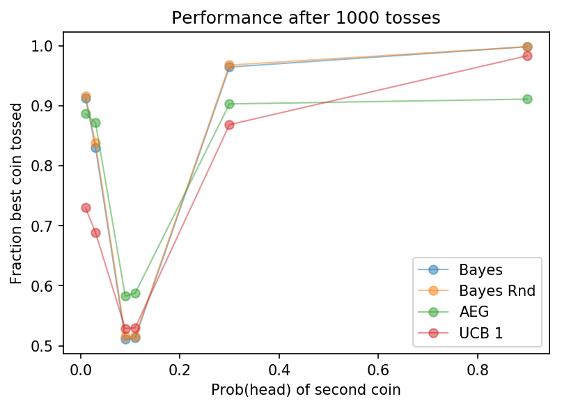
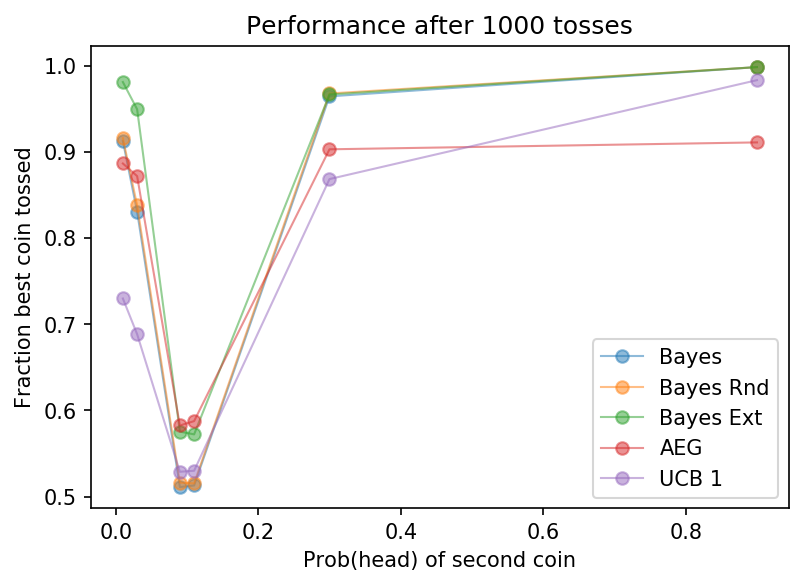
Perhaps the best measure of how well the algorithm is doing is to see how often it tosses the best coin. This measure will always lie between zero and one, so we can directly compare say a 1% coin with a 30% coin, even though we’d expect the latter to see a lot more heads.
 13
13
| Algorithm | Coin B | |||||
|---|---|---|---|---|---|---|
| 1% | 3% | 9% | 11% | 30% | 90% | |
| Bayes | 0.912 | 0.831 | 0.511 | 0.513 | 0.964 | 0.998 |
| Bayes Rnd | 0.916 | 0.838 | 0.516 | 0.515 | 0.968 | 0.998 |
| AEG | 0.886 | 0.872 | 0.582 | 0.588 | 0.903 | 0.911 |
| UCB 1 | 0.730 | 0.688 | 0.529 | 0.530 | 0.868 | 0.983 |
As is probably clear, all the algorithms fail to pick the good coin all the time when the coins are similar. Most algorithms do little better than 50%; AEG is the best of bunch tossing the good coin nearly 60% of the time.
However, when the coins can be resolved, the Bayesian algorithms are bolder in their inference and get the best score. Quantitatively, when choosing between 10% and 30% coins, both Bayesian methods choose the good coin over 95% of the time; AEG about 90% of the time.
Turning now to the final score, the basic pattern is repeated. One point is worthy of note: although the AEG algorithm does better job of distinguishing the coins when they are similar, this doesn’t make much difference to the total number of heads at the end of the run. After all, if the coins are very similar it won’t matter much which one you choose!
| Algorithm | Coin B | |||||
|---|---|---|---|---|---|---|
| 1% | 3% | 9% | 11% | 30% | 90% | |
| Bayes | 92.110 | 88.189 | 95.101 | 105.029 | 293.032 | 898.725 |
| Bayes Rnd | 92.393 | 88.782 | 95.118 | 105.175 | 293.579 | 898.513 |
| AEG | 89.786 | 91.208 | 95.923 | 105.948 | 280.570 | 828.705 |
| UCB 1 | 75.716 | 78.166 | 95.306 | 105.327 | 273.677 | 886.324 |
Perhaps the proper conclusion to draw is that you need to think carefully about the appropriate measure when evaluating the different algorithms.
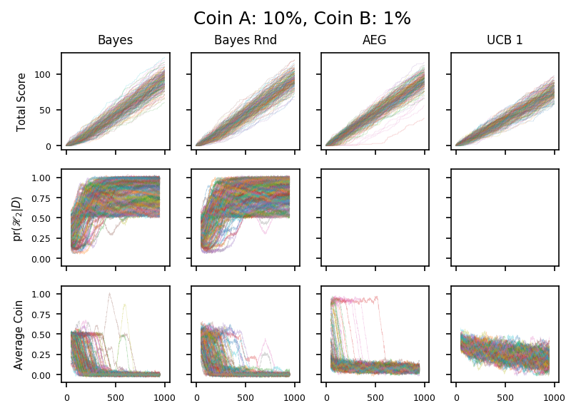
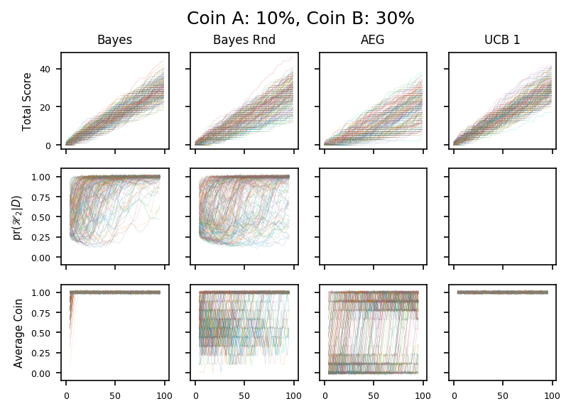
We turn now to (many) colourful plots. Each column of three plots below corresponds to a single entry in the table above and a single dot on the graph.
The first graph in each column shows the total number of heads which increases monitonically as the run progresses. The slope of the graph shows the average number of heads per toss, and I think it isn’t entirely fanciful to suggest that in some cases you can see the slope increase as the algorithm learns which coin is best.
The third graph shows which coin we are tossing. It is averaged over a small number of tosses and noise is added to make identical traces more obvious. There are clear differences in the way the algorithms work:
- The Bayesian algorithms start tossing each coin roughly 50:50, then switch almost entirely to one coin, which is almost always the better one. Before we switch, which corresponds to \(\mathscr{H}_1\) being preferred, the random variant is noisier.
- The AEG algorithm seems to embrace one coin quite quickly, but then upgrades over time if that choice seems to be wrong.
- The UCB1 algorithm stays close to 50:50, and drifts towards the correct coin en masse.
Finally, the second graph shows which model the Bayesian algorithms consider to be best. Formally, we plot the probability of \(\mathscr{H}_2\) given the data. Again we add noise to give a better representation of the probability density.
In all cases, \(\mathscr{H}_1\) and \(\mathscr{H}_2\) are equally probable a priori, and so the traces all start at 0.5. Initially we do not have enough data to support the two-paramter model and so the trace moves down, over time \(\mathscr{H}_2\) fits the data better and so the trace moves up.
When \(\mathscr{H}_2\) becomes more probable than \(\mathscr{H}_1\), we move into the exploiting phase. At this point, the better coin is tossed exclusively, so we stop learning about the other coin. If the limiting factor on being sure that we have different coins is the uncertainty about the poorer coin, then this won’t change over time. This is why the traces don’t typically proceed to \(\textrm{pr}(\mathscr{H}_2|D) = 1\), but instead fill the half-space \(\textrm{pr}(\mathscr{H}_2|D) > \frac{1}{2}\).
Finally we should also discuss the possibility that the algorithm picks the wrong coin when it switches to \(\mathscr{H}_2\). This might happen if, for example, the good coin has a run of bad luck at the beginning and is never investigated again. In practice this does happen, but apparently not often enough to affect the overall result significantly. Mitigations for this will be discussed later.
Note, that the converse problem, where the bad coin has a lucky streak isn’t as big a problem: we would keep tossing the bad coin and eventually its lucky-streak would end.
 14
14
 15
15
The two plots above correspond to the case were the second coin is much less likely to give a head. For the first coin, the difference is large enough to be identified within 1000 tosses; for the second the algorithms are still not sure.
 16
16
 17
17
These two plots show coins which are very similar. As expected the Bayesian algorithms only rarely move into the exploitation phase. In one case, it exploits the wrong coin, choosing to toss the 9% coin instead of the 10%. As discussed in the text, this mistake might persist for a long time because the algorithm isn’t tossing the 10% coin and so will persist in its delusion that it’s a bad choice.
 18
18
 19
19
Finally, these plots show how the algorithms handle the second coin being relatively very likely to land heads. It is clear that these are easier scenarios: all the algorithms swiftly pick the good coin and exploit it.
100 tosses
Below, we zoom in on the early steps of the run, looking at only 100 steps i.e. the first tenth of the run above. The plot below shows the overall performance, and as you’d expect it is somewhat worse than for the longer runs. Unsurprisingly the easy scenarios are affected less.
 20
20
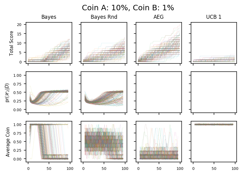
Beyond the somewhat facile observation above, there a few interesting things in the detailed evolution for the extreme coins.
 21
21
The graphs above show 1% and 10% coins. Usually, we don’t expect to resolve the difference between the coins in 100 tosses, so we expect the Bayes algorithm will often toss each coin 50 times: the data bear this out.
With this pair of coins, there is a about a 70% chance we will be in one of only ten discrete states \(n_A \in \{3,4,5,6,7\}, n_B \in \{0,1\}\). This explains the discrete lines seen in the plot of \(\textrm{pr}(\mathscr{H}_2|D)\).
The situation is similar for the Bayes Rnd algorithm but the number of times each coin is tossed is noisy, and this blurs the traces.
 22
22
Finally the plots above show an easy inference problem: the superiority of the 90% coin becomes evident in less than ten tosses. Consequently the traces here show the only times the 10% coin will be used in the entire run, even if it lasts much longer.
Note that we might remain quite uncertain about how bad the weaker coin is: we need only to know that it is weaker than the 90% coin. Having decided that we no longer toss it, and thus no longer learn about it. Given that this happens so quickly, it is likely that the long term uncertainty in the 10% coin will persist at one of the handful of values consistent with, say, \(n_A \approx 5\). This is even more obvious in the graph of \(\textrm{pr}(\mathscr{H}_2|D)\) for 1,000 tosses in the previous section.
10,000 tosses
Finally let us explore longer time scales, and look what happens when we toss the coins 10,000 times.
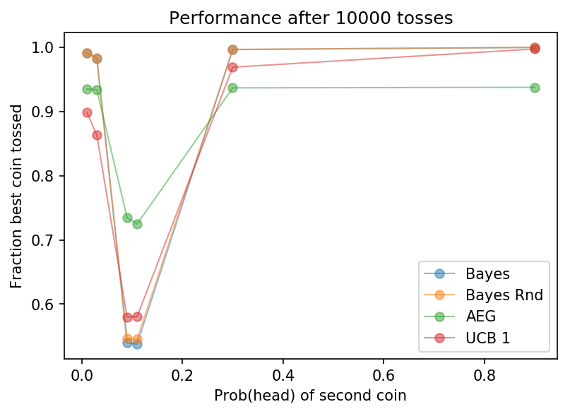 23
23
One interesting observation: the AEG algorithm still tosses the bad coin nearly 10% of the time here, which is bad for performance. Perhaps different tuning would help.
For the Bayesian algorithms, the interesting data concern the 9% and 11% coins: can we resolve the difference between one of them and the benchmark 10% coin ? Perhaps as we might expect, no!
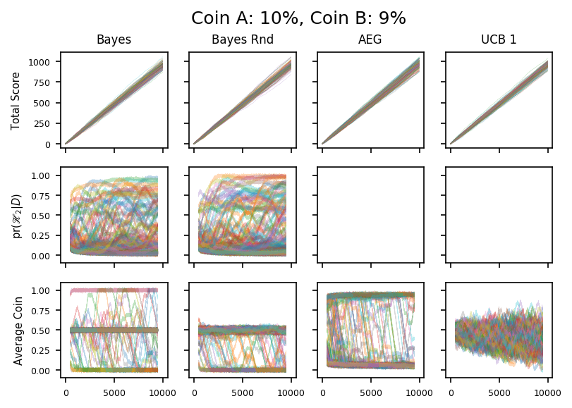 24
24
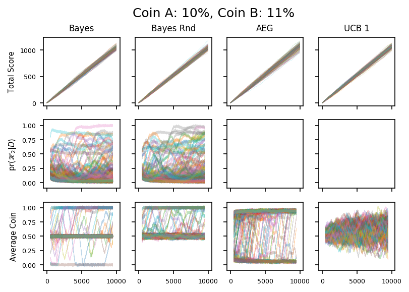 25
25
Shock response
As a final experiment with these Bayesian algorithms, let’s explore how they do when a new coin appears in the middle of a run. In the examples below, we toss the 10% coin 1,000 times letting the algorithm observe the results. Then we allow the algorithm to pick the coin, and see what happens after 100 tosses.
 26
26
In the first case, the new option is a 1% coin. As usual, the Bayes algorithm is the easiest to understand. It starts by tossing the new coin exclusively, concludes that it’s inferior after about 35 tosses, and then switches back.
\(\textrm{pr}(\mathscr{H}_2|D)\) is a useful diagnostic: it starts of at a half reflecting the equal a priori probabilities, then falls because the Occam factors prefer \(\mathscr{H}_1\) until we have enough data to support \(\mathscr{H}_2\). Note that the probability only increases very slowly once we have switched back to the 10% coin. We aren’t very sure whether we have one class or two because we don’t have enough data to characterize the second coin very well. The state persists because we have gone back to tossing the first coin.
Over longer periods, \(\textrm{pr}(\mathscr{H}_2|D)\) does rise, presumably driven by a bad run on coin A favouring \(\mathscr{H}_1\) which lets us explore coin B for a while.
 27
27
By contrast the simulation above shows what happens when then second coin is better: here a 30% coin. Although the immediate response of the algorithm is the same—toss the new coin—it rapidly becomes clear that the switch is advantageous and we keep tossing it.
In information terms this means we keep getting more information about the poorly characterized coin, and become confident that it is better. Accordingly \(\textrm{pr}(\mathscr{H}_2|D)\) climbs rapidly to one.
There is one further observation: as noted above the algorithms will start to toss the new coin immediately just because it is new. If the new coin happens to be better than the old, the algorithm might appear to be preternaturally astute by switching to the new coin so quickly. In other words, in the short-term the algorithm’s performance is dominated by whether the new coin is better or worse than the old. This care is needed to assess the algorithm’s quality here.
Extreme tossing
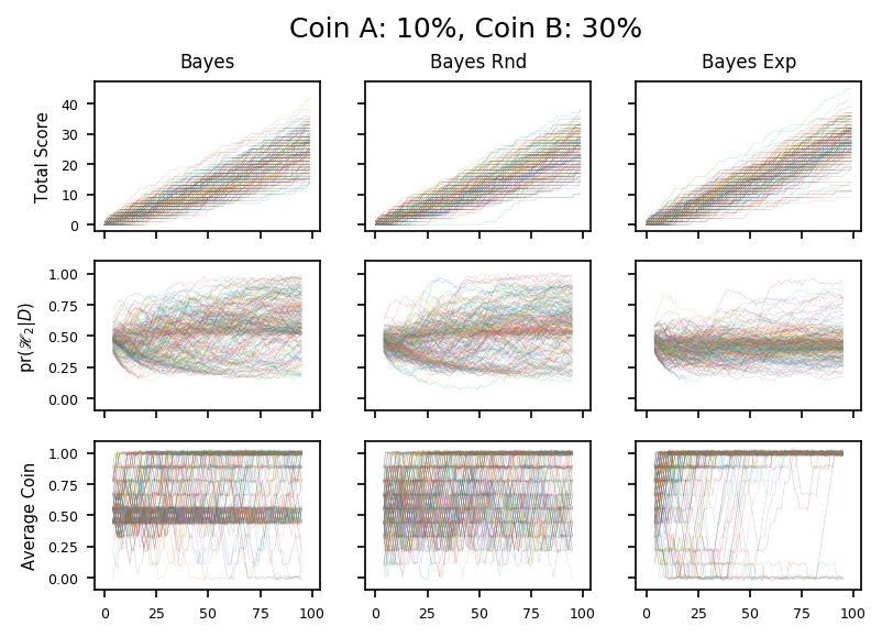
Finally I present a different algorithm, which does extremely well on the tests shown here.
 28
28
| Algorithm | Coin B | |||||
|---|---|---|---|---|---|---|
| 1% | 3% | 9% | 11% | 30% | 90% | |
| Bayes | 0.550 | 0.531 | 0.503 | 0.504 | 0.729 | 0.982 |
| Bayes Rnd | 0.560 | 0.540 | 0.505 | 0.505 | 0.750 | 0.982 |
| Bayes Ext | 0.835 | 0.766 | 0.537 | 0.539 | 0.888 | 0.982 |
| AEG | 0.694 | 0.664 | 0.525 | 0.523 | 0.779 | 0.845 |
| UCB 1 | 0.595 | 0.575 | 0.511 | 0.511 | 0.698 | 0.921 |
 29
29
 30
30
| Algorithm | Coin B | |||||
|---|---|---|---|---|---|---|
| 1% | 3% | 9% | 11% | 30% | 90% | |
| Bayes | 0.912 | 0.831 | 0.511 | 0.513 | 0.964 | 0.998 |
| Bayes Rnd | 0.916 | 0.838 | 0.516 | 0.515 | 0.968 | 0.998 |
| Bayes Ext | 0.981 | 0.949 | 0.575 | 0.572 | 0.966 | 0.998 |
| AEG | 0.886 | 0.872 | 0.582 | 0.588 | 0.903 | 0.911 |
| UCB 1 | 0.730 | 0.688 | 0.529 | 0.530 | 0.868 | 0.983 |
The algorithm is still basically a Bayesian approach: like the examples above we use Evidence ratio to choose when to switch into the exploitation phase; and to exploit we always choose the coin with the higher fraction of heads.
However, while exploring we pick the coin which is most likely to keep us in the exploring phase.
It’s time for some algebra. From above the Evidence ratio is
\[ Q(n_a, n_b) \equiv \frac{\textrm{pr}(\mathscr{H}_1|h_A, n_A, h_B, n_B)}{\textrm{pr}(\mathscr{H}_2|h_A, n_A, h_B, n_B)} = \frac{n_A + n_B + 1}{(n_A + 1)(n_B + 1)}\; \binom{n_A + n_B}{h_A + h_B} \Big/ \binom{n_A}{h_A}\, \binom{n_B}{h_B}. \]where large \(Q\) corresponds to a high probability of \(\mathscr{H}_1\).
When we toss a coin, we choose either A or B. Then the coin gives us either a head or a tail. So, after the next toss, we will be in one of four states. Assume, without loss of generality, that we pick coin A. Further, assume that the coin gives more heads than tails. Thus, we are likely to get a head on the next toss, after which the most likely state is that:
\[ \begin{eqnarray} n_A &\to& n_A + 1, \\\ h_A &\to& h_A, \\\ n_B &\to& n_B, \\\ h_B &\to& h_B. \end{eqnarray} \]It is a matter of algebra to show that,
\[ Q(n_a + 1, n_b) = Q(n_a, n_b) \, \frac{n_A + n_B + 2}{n_A - h_A + n_B - h_B + 1} \, \frac{n_A - h_A + 1}{n_A + 2}, \]swapping A & B tells us,
\[ Q(n_a, n_b + 1) = Q(n_a, n_b) \, \frac{n_A + n_B + 2}{n_A - h_A + n_B - h_B + 1} \, \frac{n_B - h_B + 1}{n_B + 2}. \]So our best guess to maximize \(Q\) after the next toss is to pick coin A when
\[ \begin{eqnarray} Q(n_a + 1, n_b) &>& Q(n_a, n_b + 1) \\\ \frac{n_A - h_A + 1}{n_A + 2} &>& \frac{n_B - h_B + 1}{n_B + 2}, \end{eqnarray} \]which after some algebra gives,
\[ \frac{h_A + 1}{n_A + 2} < \frac{h_B + 1}{n_B + 2}. \]As can easily be seen, these ratios are the fraction of heads where we add one to the count of heads and tails. It is the result you’d get from assuming a beta-distribution prior with one head and one tail, though it’s not clear to me why this is the case. Happily it is always well-behaved numerically, even before we have any data.
The analysis above assumes that we don’t get a head on the new toss: if we assume instead that we do, we get,
\[ \frac{h_A + 1}{n_A + 2} > \frac{h_B + 1}{n_B + 2}. \]One way to see this is to consider the dual problem where we consider the numbers of tails instead.
You can summarize both results by saying that to maximimize the chances of preferring \(\mathscr{H}_1\) after the next toss, we should toss the most extreme coin.
Here’s a python implementation:
log_ev1 = (log_binomial(na, ha)
             + log_binomial(nb, hb)
             - log_binomial(na + nb, ha + hb)
	     - math.log(na + nb + 1)
	  )
log_ev2 = -(math.log(1 + na) + math.log(1 + nb))

if (log_ev2 < log_ev1):
    lhs = (ha + 1) * (nb + 2)
    rhs = (hb + 1) * (na + 2)

    h = ha + nb
    n = na + nb

    if    2 * h > n:
       (u,v) = (rhs,lhs)
    elif  2 * h < n:
       (u,v) = (lhs,rhs)
    else:
      return random.randint(0,1)

    if   (u > v):
        return 0
    elif (u < v):
        return 1
else:
    if   (ha * nb < hb * na):
        return 1
    elif (ha * nb > kb * na):
        return 0

return random.randint(0,1)
Note that the code make a crude comparison to decide whether it is trying to minimize or maximize the modified fraction of heads. In cases where both coins are close to 50% this might well not work well. I have not explored this case though.
Discussion
Although the motivation for this algorithm came from looking at the likely Evidence ratio, it isn’t clear that this is the best way to look at it.
For one thing, it is empirically better to choose on the basis of the most probable future Evidence ratio rather than on the basis of its expectation.
For another, the final result is a simple ratio which could be derived in other ways: in other words there might be a different general principle which happens to give the same exploration algorithm in this case. For example, it would be interesting to see if there’s a good information theoretic justification.
Nevertheless, the algorithm appears to be locally good: not only is it better to work with the most-likely rather than the average prediction, but quantitatively \(a = 1\) appears to be the best choice for the fraction
\[ \frac{h_i + a}{n_i + 2a}. \]Half-hidden in the algorithm is the question of whether to explore or exploit when the predicted Evidence ratio is unity. Having tested both options, it seems to not matter much, which is at least consistent with the algorithm chosing an optimal time to switch.
These comments are all predicated on the particular tests shown here: before doing much more work it would be sensible to test it with different coin parameters.
Not only is there a question about the direction we should try to optimize when the number of heads and tails are similar. There is also a qualitative difference between optimizing good coins and bad: with good coins we want to keep on tossing the extreme one, with bad coins we want to swap.
Conclusions
Although it doesn’t seem to be part of the standard AB-testing repertoire, I think the Bayesian framework outlined above has much to recommend it. Not only does it give good results, it is also a principled approach in the sense that much of the algorithm comes from the direct application of more abstract mathematics.
That said, the tests here are not exhaustive and so it is premature to conclude that the results are robust with respect to the details of the problem before us.
For one thing, all the tests use a 10% coin in one arm of the comparison. This might be appropriate when we are trying to optimize an event which happens reasonable often, but we might draw different conclusions if we used a 90% coin, or indeed more extreme values: say 1% or 99%. However, this article is already rather too long, and so I’m happy to file these tasks under ‘Future Research’.
Another issue is that we have assumed the coins are stationary i.e. that the underlying probability doesn’t change. That might make sense for a coin, but it isn’t hard to imagine that the desirability of a particular advert would depend on the time of day, or the proportion of souffles which fail to rise might depend on the temperature in the kitchen. If the underlying probabilites change, then the risk is that the algorithm won’t notice because it considers the data it has already gleaned is definitive.
As such, this problem is similar to the situation where one coin has a run of really bad luck and is unfairly rejected, never to be sampled again. I can see a couple of obvious ways to tackle this: one could either impose a hard limit on how biased the tossing algorithm is, or one could expire old data.
For example, it would be easy enough to make sure that in every hundred tosses, we always toss both coins at least once. Such an approach is likely to make the average performance worse but make the worst performance better. Of course there’s nothing to say that 100 is the right number to use: it will depend on the properties of the two coins and whether we subjectively care more about the extreme or expected result.
Expiring old data seems a more direct approach to worrying about the coins’ properties changing over time. However, if the variation has some underlying structure it might be better to extend our model to capture it. Explicitly if we think the temperature matters, we might only use past data with an appropriate temperature, or replace the fixed value \(p\) in our analysis with a function of the temperature. We would need to extend our analysis, but that is conceptually straightforward.
Again it would be nice to test all this on real data in a real setting. In particular it would be nice to know and perhaps helpful if the superior performance shown by the simulations here is also found in production.
References
- 1. https://en.wikipedia.org/wiki/A/B_testing
- 2. https://en.wikipedia.org/wiki/Monte_Carlo_tree_search
- 3. https://en.wikipedia.org/wiki/Bayes%27_theorem
- 4. ./ab/rnd-1000.pdf
- 5. ./ab/rnd-10000.pdf
- 6. http://mlg.eng.cam.ac.uk/zoubin/papers/occam.pdf
- 7. ./ab/evratio-100.pdf
- 8. https://en.wikipedia.org/wiki/Stirling%27s_approximation
- 9. https://docs.scipy.org/doc/scipy/reference/generated/scipy.special.gammaln.html
- 10. http://shop.oreilly.com/product/0636920027393.do
- 11. https://github.com/johnmyleswhite/BanditsBook
- 12. https://github.com/mjoldfield/bayesian-ab
- 13. ./ab/res-1000.pdf
- 14. ./ab/paths-1000-0_01.pdf
- 15. ./ab/paths-1000-0_03.pdf
- 16. ./ab/paths-1000-0_09.pdf
- 17. ./ab/paths-1000-0_11.pdf
- 18. ./ab/paths-1000-0_30.pdf
- 19. ./ab/paths-1000-0_90.pdf
- 20. ./ab/res-100.pdf
- 21. ./ab/paths-100-0_01.pdf
- 22. ./ab/paths-100-0_90.pdf
- 23. ./ab/res-10000.pdf
- 24. ./ab/paths-10000-0_09.pdf
- 25. ./ab/paths-10000-0_11.pdf
- 26. ./ab/paths-w-100-0_01.pdf
- 27. ./ab/paths-w-100-0_30.pdf
- 28. ./ab/res-100.pdf
- 29. ./ab/cur-paths-100-0_30.pdf
- 30. ./ab/res-1000.pdf
![[ Atom Feed ]](../../atom.png "Atom Feed")