

Introduction
In his 1988 paper Bayesian Inference and Maximum Entropy1 Gull discusses how to find a lighthouse. He says:
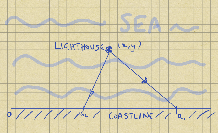
A lighthouse is somewhere off a piece of straight coastline at a position \(x\) along the coast and a distance \(y\) out to sea. It emits a series of short, highly collimated flashes at random intervals and hence random azimuths. These pulse are intercepted on the coast by photo-detectors that record only the fact that a flash has occurred, but not the azimuth from which it came. \(N\) flashes so far have been recorded at positions \(\{a_i\}\). Where is the lighthouse ?
Now, you might expect that this will be a problem about triangulation: indeed if the detectors measured the azimuths we could indeed solve it that way. However, we will have to work harder.
Formally, our task is to infer the position of the lighthouse \((x, y)\), given the position of the flashes: \( \{a_i\} \). The diagram below shows the setup:
Since Gull’s paper, the problem has been discussed in various places including Sivia’s and Skilling’s book2. The solution hasn’t changed, though these days people like to solve it3 by using MCMC packages like Stan4.
This article says nothing new either: I was interested in the problem as a test-case for demonstrating how Bayesian inference works by writing an interactive widget, and ending up writing down the algebra too.
Intuition
It is sensible to ask if this task is reasonable, so let’s start by simulating the problem. Consider a flash emitted at an angle \(\theta_1\): trigonometry shows that it will hit the coast at:
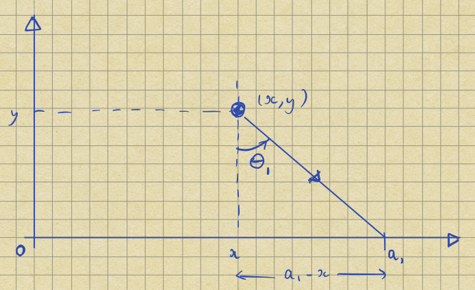
Thus we can generate representative data by picking a random angle between \([-\pi / 2, \pi / 2]\), and working out the corresponding \(a\). The histogram below shows the position of 10,000 random flashes assuming that the lighthouse’s position \((x, y) = (1, 1)\).

The most obvious feature is that we see a peak centred on \(a = 1\), i.e. the \(x\)-coordinate of the lighthouse. So, it certainly seems plausible that we’ll be able to infer \(x\): it will be roughly where the flashes arrive most often.
Now, what about \(y\) ? If we imagine scaling the diagram above around the point \((a, 0)\), then I hope it’s clear that if we move the lighthouse twice as far from the shore then the flash will move twice as far along the shore. So, as we move the lighthouse further from shore, the distribution of flashes will get twice as wide. Let’s test this by calculating a new histogram assuming that \( (x, y) = (1, 2)\):

The centre of the distribution is in roughly the same place, but the peak is broader. Although the histogram scales are the same, the central bin has only about 300 hits rather than 600 above.
Technical details
The histograms both group the observations into 100 bins spaced evenly in the range \(-10 < a < 10\). Some observations lie outside this range though: in the first example the samples ranged from about -7,000 to +2,000; in the second -12,000 to 6,000. These distributions have very wide tails!
A formal treatment
To tackle the problem formally, we need the probability of \(a\) given \((x, y)\), although the parameters are continuous so we will actually be dealing with probability densities.
Specifically, we assume that flashes are equally likely to occur in all directions and so:
\[ \textrm{p}(\theta)\,d\theta = \frac{d\theta}{\pi}. \]Remember \(\theta\) is bounded by \([ -\pi/2, \pi/2 ]\), i.e. always flashes towards the shore.
Now, using the transformation law that,
\[ \textrm{p}(a)\, da = \textrm{p}(\theta)\, d\theta, \]we have
\[ \begin{eqnarray} \textrm{p}(a) da &=& \textrm{p}(\theta)\ \frac{d\theta}{da} \, da, \\\ &=& \frac{1}{\pi} \frac{y}{y^2 + (a-x)^2} \,da. \end{eqnarray} \]This is a standard form: the Cauchy distribution5. You can see that it matches the data if we overlay it on the histogram above:

To be pedantic, the distribution is conditioned on \((x, y)\) and so we should write:
\[ \textrm{p}(a|x,y) = \frac{1}{\pi} \frac{y}{y^2 + (a-x)^2}. \]We recognize this is the likelihood6 of the arrival position \(a\) given the lighthouse’s position \((x, y)\).
Multiple flashes
It is easy to extend this to more than one flash: all are independent7 so we just see a product of the individual likelihoods:
\[ \begin{eqnarray} \textrm{p}(\{a_i\}|x,y) &=& \prod_i \, \textrm{p}(a_i|x,y),\\\ &=& \prod_i \frac{1}{\pi} \frac{y}{y^2 + (a_i-x)^2}. \end{eqnarray} \]Bayes’ theorem
Returning to our original problem, we want to infer the position of the lighthouse given the arrival locations of the flashes i.e. we want to calculate
\[ \textrm{p}(x,y|\{a_i\}). \]Happily Bayes’ theorem8 relates this to the likelihood:
\[ \textrm{p}(x,y|\{a_i\}) = \frac{\textrm{p}(\{a_i\}|x,y)\, \textrm{p}(x,y)}{\textrm{p}(\{a_i\})}. \]Our prior
As with all Bayesian inferences, we need to choose a prior9 for \((x,y)\), which represents out state of knowledge before we get any data. We hope that our conclusions will be driven by the data we receive, and so this choice won’t matter much.
In the interests of simplicity, assume a flat, bounded, prior e.g.
\[ \textrm{p}(x,y) = \begin{cases} (2d \times l)^{-1} & \text{for } -l < x < l \text{ and } 0 < y < d, \\\ 0 & \text{otherwise} \end{cases}. \]Or in other words we’re saying that we know the lighthouse is somewhere in a rectangular region, and every spot in that region is equally likely.
The posterior
Putting all of this together, if \(-l < x < l\) and \(0 < y < d\),
\[ \begin{eqnarray} \textrm{p}(x,y|\{a_i\}) &=& \left(\pi^N \times 2d \times l \times \prod_i \textrm{p}({a_i})\right)^{-1} \prod_{i = 1}^N \frac{y}{y^2 + (a_i-x)^2}, \\\ &=& \frac{1}{Z} \prod_{i = 1}^N \frac{y}{y^2 + (a_i-x)^2}. \end{eqnarray} \]Where \(Z\) absorbs all the constants, including \(\textrm{p}(\{a_i\})\) which has no \(x,y\) dependence.
Sadly it is hard to proceed analytically, but it is easy enough to compute the probability numerically on a grid and observe the results.
A demonstration
The black square above represents the area in which the lighthouse is hiding. When you click on the ‘Flash!’ button, a new flash is observed as shown in the blue bar. The square is then shaded to show the posterior probability density of the lighthouse’s position.
The colourmap shades the most probable pixel in bright yellow, even if it’s not particularly likely in an absolute sense. So you only really know where the lighthouse is when you see a small bright area.
Flashes outside the blue box are still used in the computation, but they’re shown in red at the box edge. The height of the flash mark is chosen randomly to give a better idea of the density of flashes as more arrive.
The ‘Reset’ button moves the lighthouse to a new, random, location, and throws away all the old observations.
Finally, the small blue circle shows the true position of the lighthouse. As more data arrive, the posterior density should converge on this point.
Technical details
The code generates the probabilities on a 100×100 square grid, which seems to run happily in my browser up to about 100 observations.
The browser sees a chunk of JavaScript, but the actual code is written in PureScript10.
Discussion
The posterior probability distribution encodes all the information we know about the position of the lighthouse once we’ve taken into account the information given by the arrival positions of the flashes.
Given this distribution we could compute a mean position, and a variance around that, but it isn’t obvious that this would be helpful. If you run a few demonstrations then you’ll probably see some pretty arcs and whorls of probability. Although we could calculate the mean, it wouldn’t be very representative: there is no sense in which such posteriors are well approximated by a nice little ellipse.
Happily, when we have lots of data the lighthouse’s position is tied down. Then it makes more sense to calculate and quote a mean and covariance.
(In)sufficient statistics
When we analyse data with Gaussian errors, it is often helpful to calculate the mean and variance of the data, because they contain all the information we need to do the full Bayesian analysis. In other words, we can find the parameters of the Gaussian posterior distribution from just the mean and variance of the data.
You might wonder whether the mean and variance of the data would be helpful here. It seems unlikely becuase the Bayesian analysis above gives the right answer, and it contains neither of them.
Moreover, although we can calculate the mean and variance of the particular \(\{a_i\}\) we see, the mean and variance of the underlying Cauchy distribution are not defined.
\[ \int_{-\infty}^{\infty} a\, \textrm{p}(a) \, da = \frac{1}{\pi} \int_{-\infty}^{\infty} a\, \frac{y}{y^2 + (a-x)^2} \,da, \]does not exist, and
\[ \int_{-\infty}^{\infty} a^2\, \textrm{p}(a) \, da = \frac{1}{\pi} \int_{-\infty}^{\infty} a^2\, \frac{y}{y^2 + (a-x)^2} \,da \]diverges. This issue is discussed in more detail in section 7 of Cauchy page on Random Services11, at the University of Alabama12.
Fat tails
The underlying issue here is that the Cauchy distribution has enormous weight in its tails i.e. it’s not that unlikely to receive flashes a long way down the beach.
There is a practical issue here: if we imagine having only a finite length to our detector array it is likely that we will miss some important flashes, which will lead to an underestimate of the spread of \(a\). In turn this will lead to an underestimate of \(y\).
To fix this, we’d need to modify the likelihood: conceptually easy but fiddly in practice.
Source code
The code to generate the histograms and demonstration are available on GitHub13.
References
- 1. http://bayes.wustl.edu/sfg/why.pdf
- 2. https://www.amazon.com/dp/0198568320
- 3. http://www.di.fc.ul.pt/~jpn/r/bugs/lighthouse.html
- 4. http://mc-stan.org
- 5. https://en.wikipedia.org/wiki/Cauchy_distribution
- 6. https://en.wikipedia.org/wiki/Likelihood_function
- 7. https://en.wikipedia.org/wiki/Independence_(probability_theory)
- 8. https://en.wikipedia.org/wiki/Bayes%27_theorem
- 9. https://en.wikipedia.org/wiki/Prior_probability
- 10. http://www.purescript.org
- 11. http://www.randomservices.org/random/special/Cauchy.html
- 12. http://www.math.uah.edu/stat/
- 13. https://github.com/mjoldfield/gulls-lighthouse
![[ Atom Feed ]](../../atom.png "Atom Feed")