

Preamble
If one wants to make time-lapse movies, then one really needs a device which regularly tells the camera to take a picture. Despite its active role, such things are called intervalometers.1 You can buy them ready made, and the Internet is awash with designs for DIY versions: just ask Google.2 However, I designed and built my own.
Desiderata and the broad design
I decided that the following were important to me:
- long battery life;
- easy, repeatable setting;
- good accuracy;
but that I didn’t worry too much about:
- precision;
- fancy status displays;
- non-temporal triggers.
Perhaps the key decision was the high-accuracy, low-precision trade-off. By this I mean that I want to be able to easily specify e.g. a 1 minute interval between frames, but I don’t need the ability to specify 1 minute and 3 seconds. However, when I say one minute I really do mean one minute.
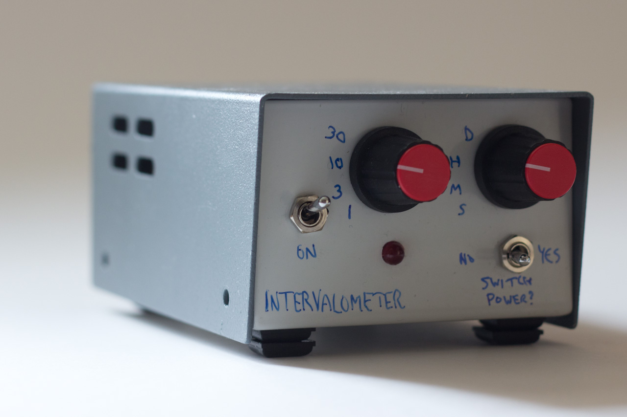
This naturally led me to a digital UI, rather than e.g. a potentiometer and some sort of display. In fact, I used a couple of 4 way switches: one specifies 1,3,10 or 30, the other seconds, minutes, hours or days. One can simply look at the positions of the switches to see how the device is configured: we don’t need a fancy LCD display.
To actually generate the pulses there are a few choices. One might distinguish between analogue solutions like the ubiquitous 555 timer, and digital ones which are effectively a quartz-oscillator and a programmable divider. The latter seem to offer better long-term stability, so that’s what I used.
For no better reason than I had some to hand, I based the device on a PIC 16F690.3 To keep the power consumption down, it’s clocked with a 32kHz quartz crystal. The whole thing is easy to power from a couple of AA batteries, but this isn’t critical. For example a 5V supply could be used instead if that were more convenient.
Finally one has to decide what to do when the time comes to take a photo. I want the intervalometer to drive a Canon 400D DSLR, which has separate focus and trigger inputs. It seems sensible to drive both of them independently, giving the camera a few seconds to focus before taking the photo. That way any variation in the time the camera takes to focus won’t affect the time at which the photo is taken.
On top of this, I wanted an extra output so that, for example, I could break the power to the camera when it wasn’t needed (the 400D draws about 40mA when ‘resting’).
In total then, then are three outputs which all all opto-isolated. I’m not sure whether this was necessary, or indeed desirable, for the camera, but still.
Finally, as you’d expect, there’s also a status LED on the front panel. Normally this is off, but it flashes when the camera’s being asked to focus then glows steadily when the shutter’s triggered.
Abstracting, our device takes a 5-bit input configuration (4 numbers × 4 units × 2 power modes) and generates a sequence of 4-bit outputs. Simples!
Hardware design
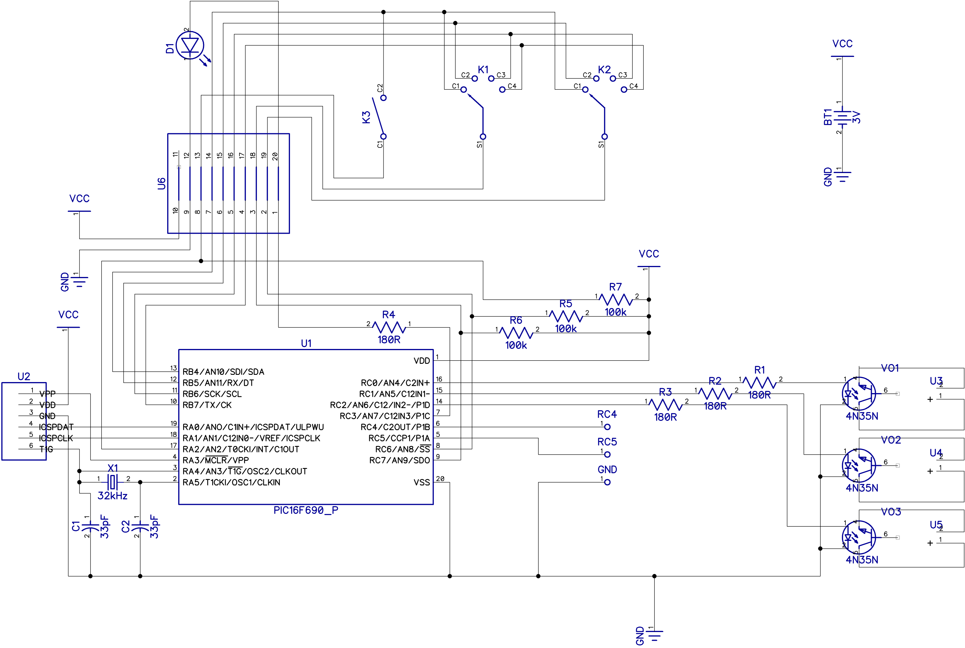
The basic schematic is shown below, exported from DipTrace.4 Feel free to play with the source code.5
 6
6
There’s very little here beyond the basic outline above. Switches K1 and K2 set the interval. To save input pins we arrange them in a matrix which we scan in software. Switch K3, an addition simply enables or disables the third output, which might be used to control camera power.
| K2 / RC6 / value | K1 / RC7 / unit | |
|---|---|---|
| RB4 | 1 | second |
| RB5 | 3 | minute |
| RB6 | 10 | hour |
| RB7 | 30 | day |
We have a couple of spare outputs on PORTC, and they’re brought out to test pads. Normally, we use RC4 to generate a calibration signal.
Finally, U2 is a standard Microchip ICSP header, suitable for a PICKit2 or similar programmer.
A prototype was built on stripboard,
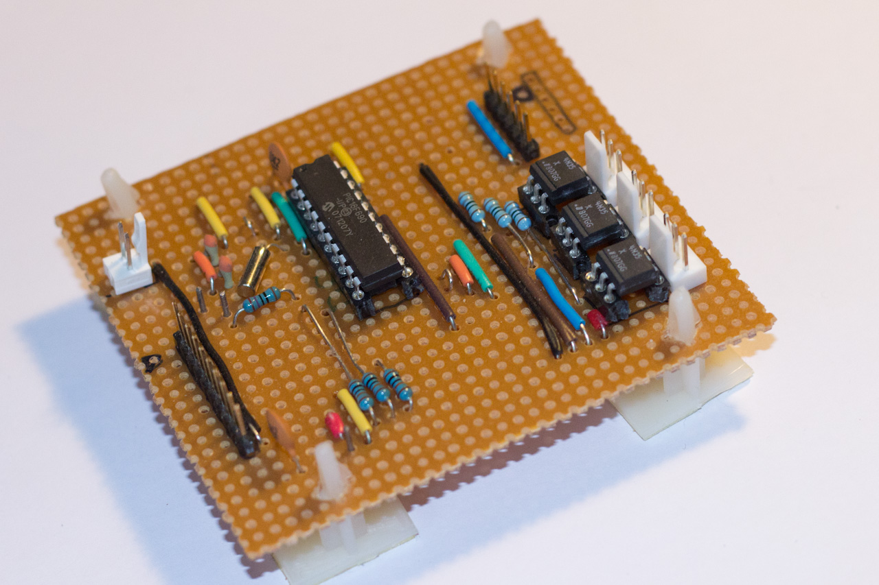
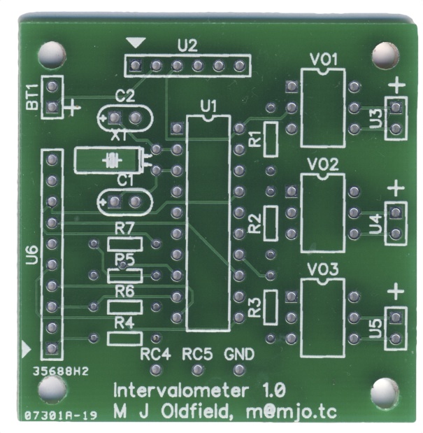
but I designed a simple PCB too. If you’d like to build your own, then you might find the gerber files7 on GitHub. As you can see, it’s a very simple PCB:
Testing
If you do build the board, it is probably wise to set the interval to 10 seconds so that you get some action fairly quickly.
There is also a useful test signal on RC5. You should see a 16kHz signal with a very low duty-cycle: the on-time is about 490µs.
Incidentally at the time of writing I have some spare PCBs. If you’d like one please let me know.
Software
The software is a simple bit of assembler compatible with GNU’s gpasm. It’s not particularly elegant or efficient, but seems to work. You can grab the source and a hex file8 from GitHub.
To understand the code, it’s helpful to know that Timer1 is configured to generate interrupts at about 16Hz, and most of the code runs inside the Timer1 interrupt. Timer1’s is clocked by the system oscillator, prescaled 4:1, and so counts at about 8kHz. Thus, it’s synchronous with the instruction clock—instructions take four ticks on this processor. To generate the 16Hz interrupts, we need 512 counts per interrupt. Incidentally 16Hz is somewhat arbitrary: it needs to be fast enough to scan the switches, but that’s about all.
When controlling the outputs it’s worth remembering that the longest interval between triggers is 30 days, or about 42 million periods of 16Hz. That’s just too much for a 24-bit counter:
\[ \begin{align} 30 \times 86400 \times 16 &= 41,472,000, \\ &\approx 2^{25.3}. \end{align} \]However we could use a 24-bit counter if we increment it at 4Hz i.e. on every fourth timer interrupt:
\[ \begin{align} 30 \times 86400 \times 4 &= 10,368,000, \\ &\approx 2^{23.3}. \end{align} \]So then there’s our basic design. Timer1 generates interrupts at 16Hz which we’ll use to scan the inputs. Every fourth interrupt we we’ll increment a 24-bit counter which controls the outputs. All the output transitions happen at small values of the counter, after which there will be a period of inactivity while we wait for things to start again.
Happily all the interesting transitions happen in the first 64s, so the state machine which drives them can deal with purely 8-bit quantities. It’s only the overflow detection which needs the full 24-bit calculation.
The transition state machine can be further simplified because The state of the status LED can be inferred from the other outputs and the clock phase. Accordingly we don’t need to explicitly list its transitions. This is both simpler and reduces the chance that the LED doesn’t reflect the true status.
If you want to understand the details of the output transitions then read the code, but basic idea is that we first ask the camera to focus, then ask it to take a picture. If we’re controlling power, then we need to apply it before focussing and turn it off again some time after taking the photo. The status LED is off when nothing’s happening then flashes progressively brighter, staying on continuously when the shutter’s triggered.
The traces below illustrate this. We begin with the standard behaviour, used when the interval’s a minute or longer. As the interval increases the featureless area to the right extends. It’s been arbitrarily truncated here.
 9
9
For shorter intervals the whole sequence is compressed. Here’s the 10s version:
 10
10
Finally the sequence used when we want to control the power11 is longer still: too long to sensibly display on the page.
Although the pictures are pretty, if you want to explore this in more detail you’re better off reading the source code.
Power consumption
One of the key things I wanted from the design was to keep the power consumption low. By putting the PIC to sleep one can get ridiculously low power consumption but it’s tricky then to keep the timer going.
In practice, when clocked at 32kHz and the supply voltage is 3V from a couple of AA batteries, the power consumption is about 60µA. If the AA based battery has a capacity of 1Ah it should last for nearly two years, which seems reasonable.
However there’s another significant power drain: the LEDs and opto-couplers draw about 5mA each when on. Each exposure clocks up about 15 LED seconds, or about 2 × 10⁻⁵ Ah. So a better model for battery life is to say that we’ll be able to take about 50,000 photos.
Although not disasterous, it’s obvious that this could be improved. The opto-isolators driving the camera might work with smaller currents, or could be replaced entirely with transistors: it’s not quite clear that the isolation is needed.
Without the optos, it makes more sense to reduce the power drawn by the status LED: either lower current, a smaller duty-cycle, or both.
Accurate timing
I mentioned above that I was keen to get reasonably good accuracy from the intervalometer. One movie I wanted to make was a clock with the frames exactly one minute apart. Then, the second hand would stay still whilst the other hands moved. If such a movie were to last a day, then we’d need an accuracy of about 1 in 10⁵.
We’ll ignore the issue of frequency drift for now, and pretend that the only problem to overcome is that the crystal’s frequency isn’t exactly 32,768 Hz. I don’t have a data sheet for the specific crystal I used, but an accuracy of ±20ppm seems to be fairly standard. That’s about twice what we’d like to achieve.
One could try to fix this in the analogue realm changing the oscillator capacitors and thus its frequency. However, it’s more sensible to handle the problem in the digital domain. We’ll need to get some sense of scale though. Recall that each instruction takes about 122µs to execute, and that the time between exposures must be an integral number of instructions.
Now, if we want to change the interval between exposures by 1ppm we’ll need to execute at least a million instructions. That will take about two minutes. In these days where so much software is written without much regard to the instruction count (because CPUs are so fast), it’s sobering to be in realm where we’re concerned with a single extra instruction every two minutes!
Quite often we’ll want the interval between exposures to be less than two minutes, so it’s clear that to get the right average exposure, we’ll have to vary the interval between exposures. For example, if the clock runs a bit fast so that we’d like (ideally) to have 512.3 ticks between exposures, we’ll choose between 512 and 513.
Now, over how many Timer1 cycles should we do the averaging ? We know that to get 1ppm adjustments we’ll need to wait about 2 minutes, which is roughly 2000 complete Timer1 cycles. Given that it’s not going to be a particularly quick process I thought it worth waiting 4096 Timer1 cycles. That should take a pleasing 256s to complete.
Explicitly we’ll have a tuning parameter between 0 and 4095, and implement a counter which counts from 0 to 4095. When the sum of the two is more than 4095 then we’ll load the timer with the higher number.
There’s one minor twist: rather than have a 12-bit counter (2¹² = 4096) which increments one digit at a time, there’s a 16-bit counter which counts up 16 at-a-time. Putting the four unused bits at the least-significant end means that we can specify the instruction count for the 256s cycle in a single 32-bit value.
In 256s we’ll execute about two million instructions, so our precision will be about 0.5ppm. Happily, my bench timer claims an accuracy of 0.2ppm which gives us a good way to do the tuning. To drive the timer, we’ll pulse one of the spare PORTC outputs every 256s.
There are a couple of details to consider. All the counters increment and things happen when they overflow. So, if we want n cycles in our 256s period the configuration datum will be 0x100000000 - n.
Loading a new value into Timer1 costs a couple of ticks, so actually the datum will be 0x100020000 - n.
Finally time, and instructions, will elapse between the interrupt being triggered and us reloading the timer. So, we should add a correction to the timer’s LSB rather than setting it.
In practice this scheme works well enough. Rather lazily though, there’s no convenient way to calibrate the intervalometer: instead one has to edit the constant in the source code, assemble, and upload it. Here’s the relevant code:
;; higher number => shorter period
constant	tmr1_dh   = 0xfe ; 0xfe00 -> 0x10000 = 512 => 16Hz fast clock
constant	tmr1_dl   = 0x01 ; these 2 cycles are lost when we reload

;; tweak setting (only the 12 most significant bits matter)
;; this is device/crystal specific
constant	tmr1_adj_h = 0xff ;
constant	tmr1_adj_l = 0x70 ;

;; increment to adjustment clock (0x80 => 32s cycle, 0x40 = 64s cycle, ..)
constant	adj_clk_inc = 0x10
We’ll see later that the oscillator frequency depends a bit on the supply voltage, so irritatingly if we program the PIC at 5V but deploy the intervalometer at 3V we’ll have to take this into account.
A helpful shuffle
Whilst the scheme above works, there’s a snag. All of the (n+1) cycle periods are clumped together. This makes the deviation from the ideal behaviour worse than it need be.
Happily, it’s easy to make a significant improvement. Recall that the heart of the problem is that the code for picking the Timer1 period is:
inc = (cycle + offset) > 4096 ? n : n + 1;where cycle counts from 0 to 4095, and offset is fixed.
Suppose we change that to:
inc = (P(cycle) + offset) > 4096 ? n : n + 1;where P(i) shuffles the numbers [0,4095]. Over a complete cycle the test will be true just as often, but it will be true at different times.
One could imagine all manner of clever definitions for P, but this doesn’t do a bad job:
P(i) = i `xor` ((i && 0xff) << 8)That is, just XOR the high byte with the low.
It’s probably obvious that this just shuffles the elements, but if it’s not here’s a demonstration (in Haskell):
> :m Data.Bits Data.List
> let states = [ (h,l) | h <- [0..255], l <- [0,16..255] ]
> take 8 states
[(0,0),(0,16),(0,32),(0,48),(0,64),(0,80),(0,96),(0,112)]
> let states' = map (\(h,l) -> (h `xor` l, l)) states
> take 8 states'
[(0,0),(16,16),(32,32),(48,48),(64,64),(80,80),(96,96),(112,112)]
> sort states' == sort states
True
Or, if you prefer pictures, the plot below shows the shuffle. It might make more sense to think of the plot as a bit map in which every row and column has precisely one cell filled. To see which cycles will enjoy the extra timer tick, mentally draw a horizontal line at the relevant level. Then regard the x-axis as time: if there’s a dot below the line at that time, then we’ll get an extra tick.
By contrast, the unpermuted code would simply have a ‘y = x’ line here: if you play the same game with the horizontal line, all the extra-tick times will be clumped at the left-side of the graph.

Ultimately of course we care about the effect on the interval between shutter triggers. The plots below show these, but some interpretation is needed.
Suppose we just plotted the interval over time. The interval’s nominally 10s, and we’re looking for changes on the order of 100µs: the time to execute an instruction. Clearly we’re looking for a small effect!
If there were no oscillator drift, we could simply pick the a suitable but sadly that’s not the case. The oscillator does drift over time, so we pre-process the signal to remove this. Explictly we plot the difference between the measured time and the local (±3 samples) minimum. This should remove the drift in both the intervalometer’s oscillator and the meter’s timebase (the latter might be significant because I took the measurements with an Arduino).
Rather than plot the difference in seconds, we’ll show it in clock ticks i.e. 2⁻¹³s. Despite appearances to the contrary, there’s no rounding to the nearest integer: if you look at the data you’ll see variation at the ±0.03 instruction level.
It’s immediately obvious that the XOR instruction improves the distribution: there are only two different intervals and they vary by a single instruction. By contrast the niave code sometimes generates an interval some nine ticks longer. Before we lose perspective though, that’s about one millisecond!

The XOR code isn’t perfect though. The plot below shows a small section of fifty intervals, and it’s obvious that the longer intervals aren’t quite evenly distributed over time. There are better solutions, but most need significantly more than one single instruction.

Oscillator drift
Although it would be nice to ignore it, in practice the oscillator frequency does depend on the environment.
Voltage dependence
It’s easy to verify that the frequency depends on the intervalometer’s supply voltage, and that higher voltages correspond to higher frequencies.
The graph below shows some experimental data covering the range 3–5 volts. You’ll see that the interval was measured twice at each voltage, in an attempt to isolate the voltage dependence from e.g. coincidentally correlated changes in temperature. Given that the difference between the two measurements is much smaller than the change between successive voltages, we seem fairly justified to claim that it’s voltage driving this.

It’s clear that the relationship is roughly linear, and a simple least-squares fit gives:
\[ \tau(V) = 255.99786 \left(1 - 1.12 × 10^{-6} (V - 4.0) \right). \]The basic story though is that over this range of voltages, there’s an approximately-linear fractional-change of about -1.12 × 10⁻⁶ per volt.
Thus as the battery discharges we’ll see a drop of less than 0.5V, which translates to a fractional-change of about 5 × 10⁻⁷, so we don’t have to worry about it.
On the other hand, if we program the PIC at 5V but deploy at 3V we’ll expect the period to rise by about 0.6ms. Accordingly we should tune for 255.9994s under 5V to see 256.0000s at 3V.
Temperature dependence
Quartz oscillators rely on the piezo-electric property of quartz to connect its electrical and mechanical properties: it turns a physical resonance into an electrical one. Accordingly we’d expect temperature, which changes the physical characteristics to change the electrical ones too.
Typically data sheets say that the resonant frequency change with temperature is well-modelled by,
\[ \frac{f_{res}(T)}{f_0} = 1 - \alpha (T - T_0)^2, \]where \( \alpha \approx 0.04 \times {10}^{-6} \textrm{C}^{-2} \), \( T_0 = 25^{\circ}\textrm{C} \).
Given that the effect is small, it’s easy to convert this into an expression for the period:
\[ \tau_(T) = \tau_0 \left(1 + \alpha (T - T_0)^2\right). \]Sadly I don’t have any sort of temperature controlled chamber to hand, so I just left the intervalometer on the bench for a while, logging the period and temperature automatically. Here’s what I found:

The solid line is a parabola fitted to the data by eye. It has equation:
\[ \tau(T) = 255.99929 \left(1 + 3.5 \times 10^{-8} (T - 19.75)^2\right). \]That seems broadly consistent with what we’d expect though the temperature of the extremum seems lower than I’d expected.
It seems foolish to infer too much of a quantitative nature from these data: they’re just not good enough:
- The temperature measurements are only precise to the nearest 0.5°C, and could easily have have a few degrees of systematic inaccuracy.
- The time measurements appear to have an interesting likelihood structure which probably comes from the algorithm used by the counter (a TTi TF930). For example, one sees a gap of about 50µs between the clusters of points at given temperature. That’s roughly the period of a 16kHz clock: two ticks of the intervalometer’s master oscillator or about half an instruction. Neither of those seem a particularly good explanation.
Overall though, it seems reasonable to say that if we’d expect if the temperature remains within 20±5° C the clock won’t vary by more than about 1ppm. In other words, providing we’re not working outside, we can forget about the problem.
Useful files
The project files12 are now on GitHub.
The design is available under the CCSA 3.0 license:13
A gratutitous movie
Acknowledgements
I am grateful to Peter Mann who built one of these, despite a lack of clear instructions. The article has now been improved by Peter’s feedback.
References
- 1. http://en.wikipedia.org/wiki/Intervalometer
- 2. http://www.google.com/search?q=diy+intervalometer
- 3. http://www.microchip.com/wwwproducts/Devices.aspx?dDocName=en023112
- 4. http://www.diptrace.com/index.php
- 5. http://www.mjoldfield.com/atelier/2011/08/intervalometer/prod-0.1.dch
- 6. http://www.mjoldfield.com/atelier/2011/08/intervalometer/schematic-big.png
- 7. https://github.com/mjoldfield/into-meter
- 8. https://github.com/mjoldfield/into-meter
- 9. http://www.mjoldfield.com/atelier/2011/08/intervalometer/unpowered.svg
- 10. http://www.mjoldfield.com/atelier/2011/08/intervalometer/unpowered10.svg
- 11. http://www.mjoldfield.com/atelier/2011/08/intervalometer/powered.svg
- 12. https://github.com/mjoldfield/into-meter
- 13. http://creativecommons.org/licenses/by-sa/3.0/
![[ Atom Feed ]](../../atom.png "Atom Feed")